Check The Performance of A Rooting Method Using Minimal Ancestor Deviation (MAD)

Simple demonstration how mad works

MAD: root the tree by Minimal Ancestor Deviation (MAD) See Tria et al. (2017)

knitr::opts_chunk$set(echo = TRUE)

rm(list=ls())
pathV <- "/Users/cactus/OneDrive\ -\ Aarhus\ Universitet/PhyloSynth/Backbone/BackboneV2/"
library("ape")
suppressWarnings(suppressMessages(library("phytools")))
source(paste0(pathV,"mad.R", sep="")) #source "mad" function

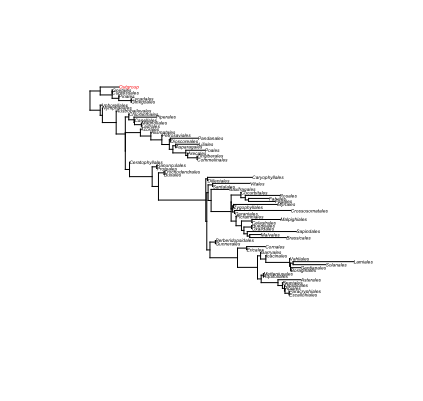
Plot original tree

tree1 <- ladderize(read.tree(paste0(pathV,"Backbone351order_species_order.tre", sep="")))
is.rooted(tree1)
plot.phylo(tree1, cex=0.3, tip.color=ifelse(tree1$tip.label %in% "Outgroup", "red", "black"))

Plot unroot tree

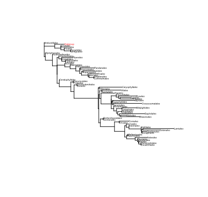
tree2 <- ladderize((unroot.phylo(tree1)))
is.rooted(tree2)
plot.phylo(tree2, cex=0.3, tip.color=ifelse(tree2$tip.label %in% "Outgroup", "red", "black"))

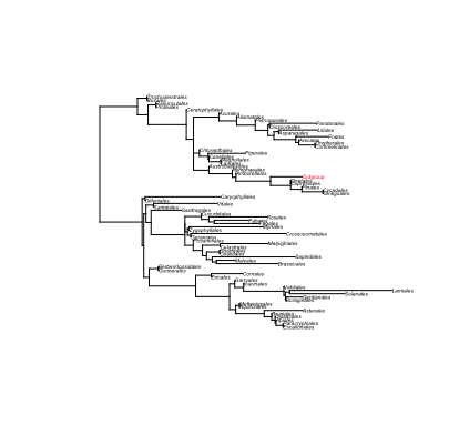
Plot the same tree rooted with MAD

tree3 <- mad(tree2)
tree3 <- ladderize(read.tree(text = tree3))
is.rooted(tree3)
plot.phylo(tree3, cex=0.3, tip.color=ifelse(tree3$tip.label %in% "Outgroup", "red", "black"))

Group picture — cheese

par(mfrow=c(1,3))
plot.phylo(tree1, cex=0.3, tip.color=ifelse(tree1$tip.label %in% "Outgroup", "red", "black"), main="original")
plot.phylo(tree2, cex=0.3, tip.color=ifelse(tree2$tip.label %in% "Outgroup", "red", "black"), main="unroot")
plot.phylo(tree3, cex=0.3, tip.color=ifelse(tree3$tip.label %in% "Outgroup", "red", "black"), main="mad.root")

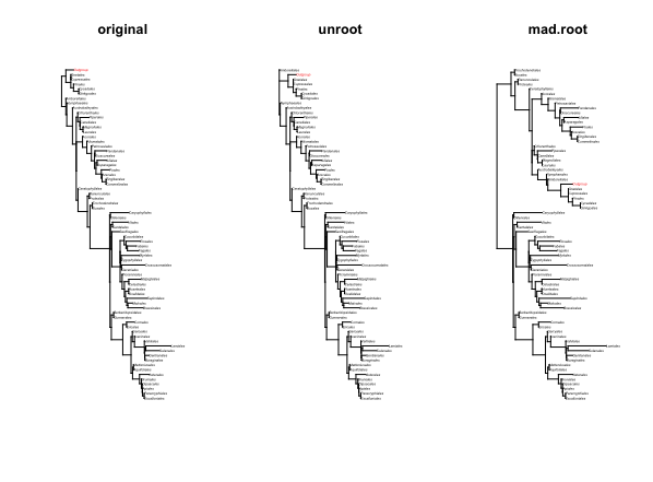
Well, visually that straightfoward as we usually see Outgroup, but I think it did a good job in terms of minimal ancestor deviation as rooting criteria.

Another example

# R package "ape" root
Tg6689 <- read.tree(paste0(pathV,"./g6689.raxml.rba.raxml.supportFBP", sep=""))
is.rooted(Tg6689)

if(is.rooted(Tg6689)){
  Tg6689a <- unroot(Tg6689)
  is.rooted(Tg6689a)
}

Outgroup <- c("Isoetes_tegetiformans_1kp", "Selaginella_apoda_1kp")

Tg6689b <- root(Tg6689a, Outgroup, resolve.root = TRUE)

is.rooted(Tg6689b)


# unroot
Tg6689.u <- unroot(Tg6689)

is.rooted(Tg6689.u)

# MAD root
tmp <- mad(Tg6689.u)

Tg6689.mad <-  ladderize(read.tree(text = tmp))

is.rooted(Tg6689.mad)

# reroot by phyx `pxrr`

Tg6689.phyx <- read.tree(paste0(pathV,"./g6689.supportFBP.rt.tre", sep=""))

is.rooted(Tg6689.phyx)

# Plot all together
par(mfrow=c(1,4))
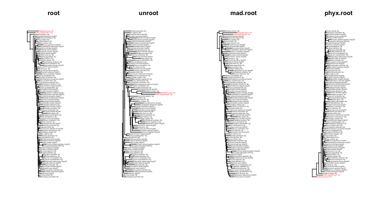
plot.phylo(Tg6689b, cex=0.3, tip.color=ifelse(Tg6689b$tip.label %in% Outgroup, "red", "black"), main="root")
plot.phylo(Tg6689.u, cex=0.3, tip.color=ifelse(Tg6689.u$tip.label %in% Outgroup, "red", "black"), main="unroot")
plot.phylo(Tg6689.mad, cex=0.3, tip.color=ifelse(Tg6689.mad$tip.label %in% Outgroup, "red", "black"), main="mad.root")
plot.phylo(Tg6689.phyx, cex=0.3, tip.color=ifelse(Tg6689.phyx$tip.label %in% Outgroup, "red", "black"), main="phyx.root")

Discussion

So apparently, phyx is better. Rooting via MAD may not be always straightfoward as other methods with a clear outgroup id. Moreover, the same outgroup, the branch length may be different in different gene trees. Since different genes have different evolution rates, then branch length may vary from gene to gene, hence likewise the ancestor deviation also vary.

Overall, I still think rooting via mad is usefull under certain circumstances. For instance, if you have a bunch gene trees have 0 outgroup sampled, and some downstream analyses required rooted trees, then MAD did provide a decent root. Other common methods require to provide an outgroup. For example, phyx function pxrr requires a ranked (-r) comma-seperated outgroups by -g (see here); but it did not provide a solution for the scenarios that if no outgroup sampled at all for some genes. Some other package (e.g., Newick Utils) will use the longest branch as root, but long branch could be misled as well.